Usage and Examples
This guide explores a few more complicated tasks one might wish to use this code for.
- Reproducing the line profile and transfer function shown in CM96
- Reproducing sample cloud model results from Pancoast+2014
- Reproducing the line and phase profiles shown in Long+2023
- Predicting BLR sizes from differential visibility amplitudes
- Reproducing the combined model line and delay profiles shown in Long+2025
- Defining your own custom models
- Multi-line models
- Velocity-resolved line ratios
- Running on the GPU
- Additional (selected) helpful tools from the API not described above
Reproducing the line profile and transfer function shown in CM96
CM96 showed that disk-wind models of the BLR could produce single-peaked line profiles, and as part of their results they generated a hypothetical 2D transfer function for a disk-wind BLR as applied to NGC 5548. We can reproduce such a map with just a few lines of code using BroadLineRegions.jl.
BroadLineRegions.jl exports itself as both BroadLineRegions and the shorter BLR. We will use the shorter BLR throughout these examples but know that BLR is equivalent to BroadLineRegions should you prefer the longer version.
First, let's define the model using DiskWindModel:
using BroadLineRegions
mCM96 = BLR.DiskWindModel(3000.,100.,1.,75/180*π,
        nr=2048,nϕ=1024,scale=:log,f1=1.0,f2=1.0,f3=0.0,f4=0.0,
        I=BLR.DiskWindIntensity,v=BLR.vCircularDisk,τ=5.0,reflect=false)
We use the parameters from CM96 for $\bar{r} = 3000\rm{r_s}$, $r_{\rm{fac}} = 10^2$, $\alpha = 1$, and $i = 75^{\circ}$. CM96 considered the case of radial and Keplerian shear only, so we turn these gradients on by setting $f_1 = 1$ and $f_2 = 1$ (radial and Keplerian shear, respectively) and turn off the remaining velocity gradients by setting $f_3 = 0$ and $f_4 = 0$.
To have a well sampled model grid we pick nr=5096 and nϕ=1024 with scale=:log, which will result in the returned model object having 5096 "rings" in our circular camera aperture with each ring holding 1024 grid cells evenly divided in $\phi$ space.
While this is the default, for the sake of this demonstration we also set I=BLR.DiskWindIntensity to explicitly tell the model to use the intensity formulation first proposed in CM96 (and using the "f" parameter language introduced in Long+2023). We also tell the model to calculate the velocities according to the built in function BLR.vCircularDisk, which simply calculates the projected line of sight velocity as $v = \sqrt{\frac{\rm{r_s}}{2r}}\sin i \sin\phi$.
Finally, while not required, we set τ = 5.0 as we want our disk to be optically thick and reflect = false as we do not want to move any points from the back to the front.
Now that we have a model, let's get the line profile and store it in our model:
p = BLR.getProfile(mCM96,:line,bins=101) #get the line profile using 101 bins in velocity-space, otherwise using default params
BLR.setProfile!(mCM96,p) #store the line profile in our model structure
We can do a quick visualization with the built-in profile macro:
BLR.profile(mCM96) #plot all profiles stored in model object, here we only have set :line so only :line will be plottedWhich should return a plot like this (left panel, right panel is Figure 2 in CM96):
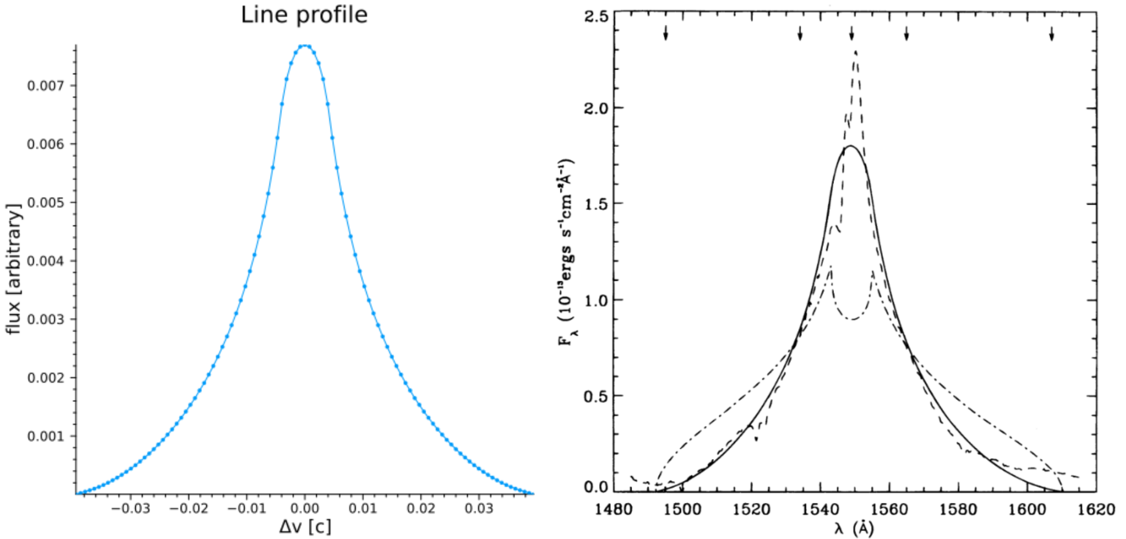
Note that the y-axis units are arbitrary and the x-axis is in units of velocity [$c$], not $\lambda$ as published in Fig 2 of CM96, but the shape clearly matches their result that the line profile for such a model should be single-peaked. This is also showing only the full model line profile (thei solid line), not the data or other models. We could reproduce their plot exactly by rescaling our flux and converting from velocity-space to wavelength space as well as plotting the data and a model line profile with azimuthally isotropic emission, but we will leave that as an exercise for the motivated reader...
It is similarly easy to use BroadLineRegions.jl to generate transfer functions for any user-defined model. In looking at Figure 4 of CM96 we see that their y-axis (delays) spans 0-20 days and the x-axis (projected velocity) -12-12 ($10^8$ $\rm{cm}$ $\rm{s}^-1$). To match our model result to theirs, we first need to convert our units of $\rm{r_s}$ to the more physical unit of days. CM96 used $M_{\rm{NGC5548}} \approx 10^8 \rm{M_{\odot}}$, which means we can calculate the conversion factor as:
M = 1e8*2e30 #kg
rs = 2*M*6.67e-11/9e16 #2GM/c^2
rsDay = rs/3e8/3600/24 #days
We only need to obtain the transfer function $\Psi$ over the range shown in CM96, so let's define the tEdges and vEdges we want to use to match their result and then generate the transfer function:
tEdges = collect(range(0.0,stop=20.0/rsDay,length=101)) #will generate 100 bins, convert 20 days upper limit to units of rs
vEdges = collect(range(-0.04,stop=0.04,length=101)) #0.04c ~12*1e8 cm/s
Ψ = BLR.getΨ(mCM96,vEdges,tEdges) #obtain transfer function with our supplied bin edges
Note that in Fig. 4 of CM96 the edges between the colors are sharp, indicating that they used discrete bins in their image to better showcase structure. While these levels are not explicitly supplied in the paper, we can make a good guess that they are somewhat evenly spaced logarithmic bins. To transform our $\Psi$ to match their binning, we can do something like:
function getΨMatch(ΨBinned,levels=[-0.4*i for i=0:11]) #generate constant log10 bins of Ψ
    #fills intervals that are closed at the top;
    #that is, for regions z1 and z2 the filled region is z1 < Z <= z2"

    logΨ = log10.(ΨBinned)
    res = zeros(size(logΨ))
    mask = (logΨ .<= levels[2]) .& (logΨ .>= levels[1])
    res[mask] .= (levels[1]+levels[2])/2
    for i=2:length(levels)-1
        mask = (logΨ .< levels[i]) .& (logΨ .>= levels[i+1])
        res[mask] .= (levels[i]+levels[i+1])/2
    end
    mask = (logΨ .< levels[end])
    res[mask] = logΨ[mask]
    return res
end
ΨDiscrete = getΨMatch(Ψ./maximum(Ψ)) #normalize and generate discrete bins
All that's left to do now is visualize the result, which we will do with the heatmap function from Julia's Plots.jl:
using Plots

heatmap(vEdges.*3e10/1e8,tEdges.*rsDay,ΨDiscrete',
    ylims=(0,20),xlims=(-12,12),clims=(-4.4,0.0),cbar=false,
    xlabel="v (10⁸ cm/s)",ylabel="τ (days)",minorticks=true,
    tickdirection=:out,widen=false,size=(500,500))
Which should return something like this (left plot, right plot is Fig 4. in CM96):
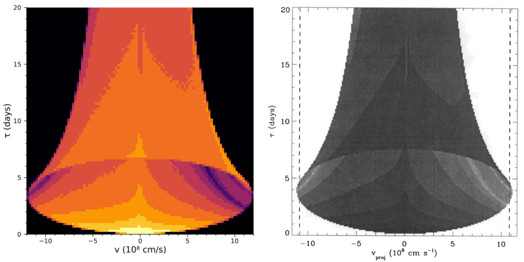
While our binning is a little off/coarser than in CM96, this is clearly a pretty good match for a quick and dirty calculation.
A few final notes:
- Note that when plotting we use
ΨDiscrete'because heatmap expects the shape of the image variable to be flipped from howBroadLineRegions.jlcalculates it (the shape ofΨwhen returned is (number of velocity bins, number of t bins)). - If you wanted to generate just the 1D response function as shown in CM96 Figure 5,
BroadLineRegions.jlhas syntax for that too:tCenters, Ψt = BLR.getΨt(mCM96,101,10/rsDay).
Reproducing sample cloud model results from Pancoast+2014
We can also generate "cloud"/thick-disk models of the BLR similar to Pancoast+2014 easily with BroadLineRegions.jl. In this section we will reproduce part of Figure 4 in Pancoast+2014, which shows five different model BLRs and their 1D transfer functions with the following parameters:
| parameter | model 1 | model 2 |
|---|---|---|
| $r_{\rm{mean}}$ [days] | 4.0 | 4.0 |
| $F$ | 0.25 | 0.25 |
| $\beta$ | 1.0 | 0.8 |
| $\theta_o$ [deg] | 40 | 30 |
| $i$ [deg] | 20 | 20 |
| $\kappa$ | -0.4 | -0.4 |
| $\gamma$ | 5.0 | 5.0 |
| $\xi$ | 0.3 | 0.1 |
| $f_{\rm{ellipse}}$ | 0.0 | 1.0 |
| $f_{\rm{flow}}$ | 0.0 | - |
| $\theta_e$ [deg] | 0.0 | - |
| $\sigma_{\rm{turb}}$ | 0.0 | 0.0 |
First, we initialize model structs for both of these cases:
M = 10^(6.5)*2e30 #kg, from Pancoast+2014
rs = 2*6.67e-11*M/9e16 #2GM/c^2, m
rsDay = rs/3e8/3600/24 #days^C #days -- model expects μ in units of rₛ
nClouds = 100_000 #small number of clouds just for demonstration
mP1 = BLR.cloudModel(nClouds,μ=4/rsDay,F=0.25,β=1.0,θₒ=40/180*π,i=20/180*π,
        κ=-0.4,γ=5.0,ξ=0.3,fEllipse=0.0,fFlow=0.0,θₑ=0.0,σₜ=0.0,
        σρc=0.0,σΘᵣ=0.0,σΘc=0.0,σρᵣ=0.0,
        I=BLR.cloudIntensity,v=BLR.vCloudTurbulentEllipticalFlow,τ=0.0)
mP2 = BLR.cloudModel(nClouds,μ=4/rsDay,F=0.25,β=0.8,θₒ=30/180*π,i=20/180*π,
        κ=-0.4,γ=5.0,ξ=0.1,fEllipse=1.0,σₜ=0.0,
        fFlow=0.0,θₑ=0.0,σρc=0.0,σΘᵣ=0.0,σΘc=0.0,σρᵣ=0.0,
        I=BLR.cloudIntensity,v=BLR.vCloudTurbulentEllipticalFlow,τ=0.0)
Where the first argument passed to cloudModel is the number of clouds to generate (here we use a relatively small number just for demonstration purposes), and the keyword arguments supplied mostly correspond to the values in the table above and are fully described in Pancoast+2014. The extra keyword arguments set to 0 but not in the table are options not used in this calculation, and the final line specifies that we would like the intensity calculated with the cloudIntensity function, the velocities calculated with vCloudTurbulentEllipticalFlow, and that the optical depth of the cloud is 0.
To compare to Figure 4 in Pancoast+2014 we can again generate transfer functions for both models:
using Plots

vEdges = collect(range(-0.015,stop=0.015,length=51)) #Δλ/λ ~ v/c
tEdges = collect(range(0.0,stop=20.0/rsDay,length=51))
Ψ1 = BLR.getΨ(mP1,vEdges,tEdges)
Ψ2 = BLR.getΨ(mP2,vEdges,tEdges)
p1 = heatmap(vEdges.*3e5,tEdges.*rsDay,(Ψ1'./maximum(Ψ1)).^(1/2),ylims=(0,20),cbar=false,
    xlabel="Δv (km/s)",ylabel="Lag (days)",minorticks=true,tickdirection=:out,
    widen=false,size=(500,500),guidefontsize=18,tickfontsize=16)
p2 = heatmap(vEdges.*3e5,tEdges.*rsDay,(Ψ2'./maximum(Ψ2)).^(1/2),ylims=(0,20),cbar=false,
    xlabel="Δv (km/s)",ylabel="Lag (days)",minorticks=true,tickdirection=:out,
    widen=false,size=(500,500),guidefontsize=18,tickfontsize=16)
Which should produce something like the left column of plots in the comparison below (top plot = p1 and bottom = p2):
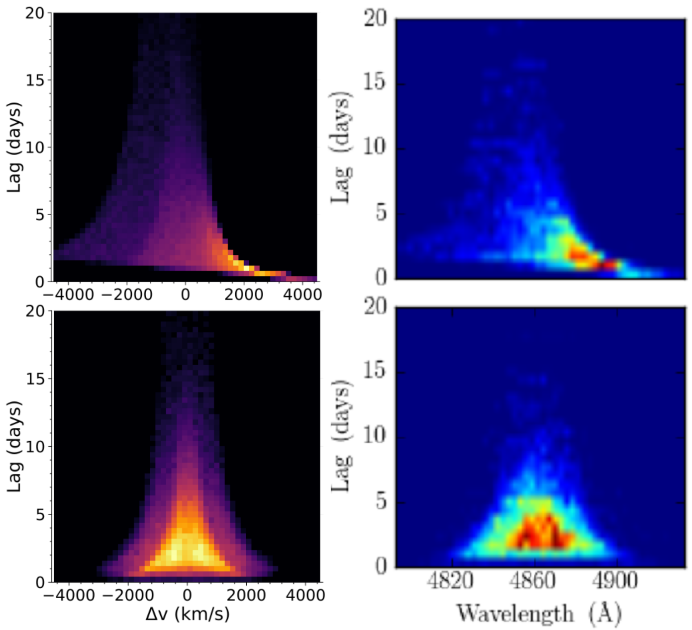
Note that again we are just trying to roughly match the color scale by eye, but the general shape and morphology looks good.
We can also quickly visualize the geometry of the system from any angle (i.e. to compare to the rightmost panel of Fig. 4 in Pancoast+2014) using the built-in plot3d macro:
BLR.plot3d(mP1,:I,cam=(10,10)) #visualize the system with points colored by their intensity with a camera at 10 deg azimuth and altitudeIterating this over a wide variety of camera angles one can produce fun 3D visualizations of the BLR models like the gifs below:
| model 1 | model 2 |
|---|---|
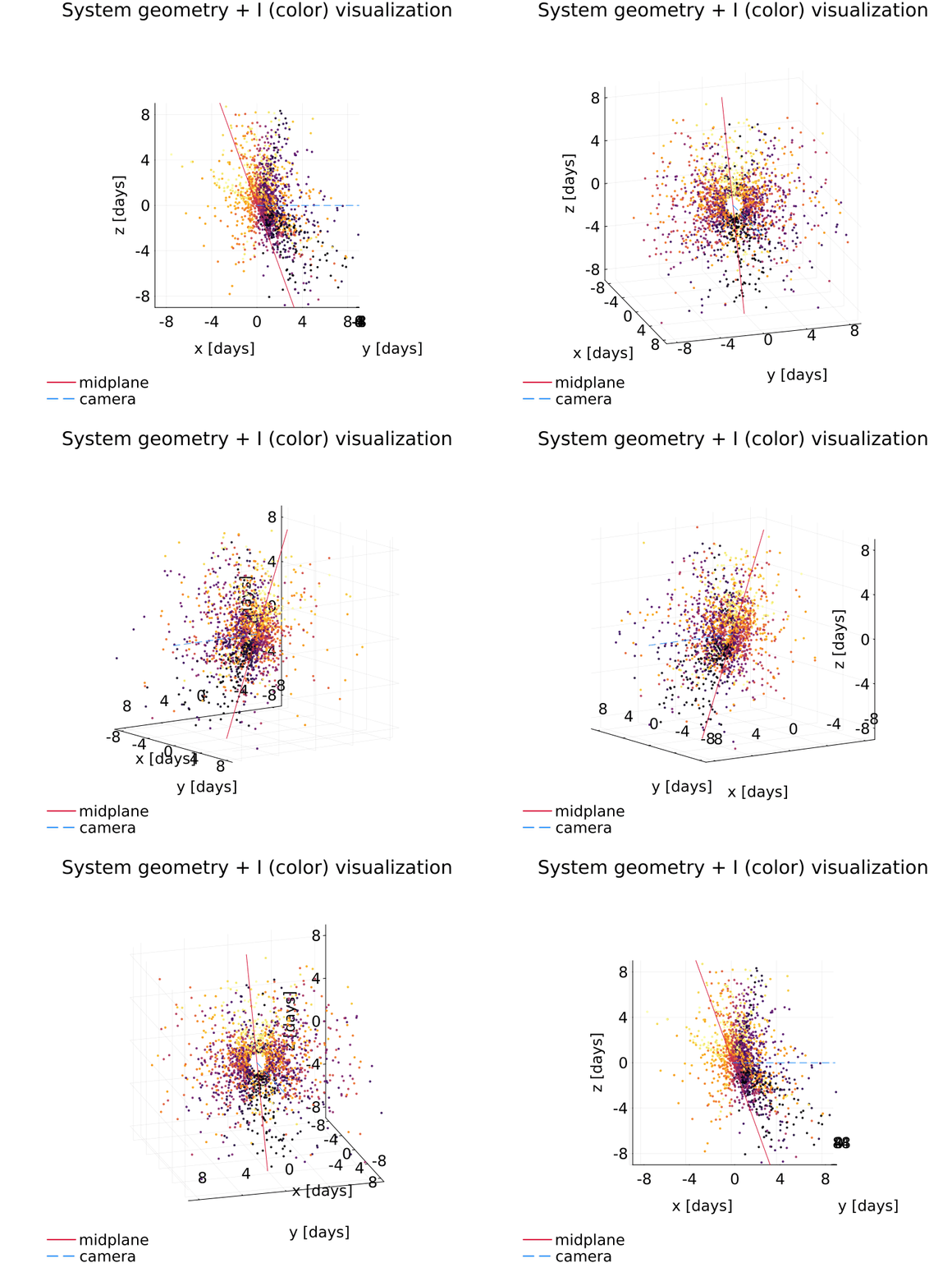 | 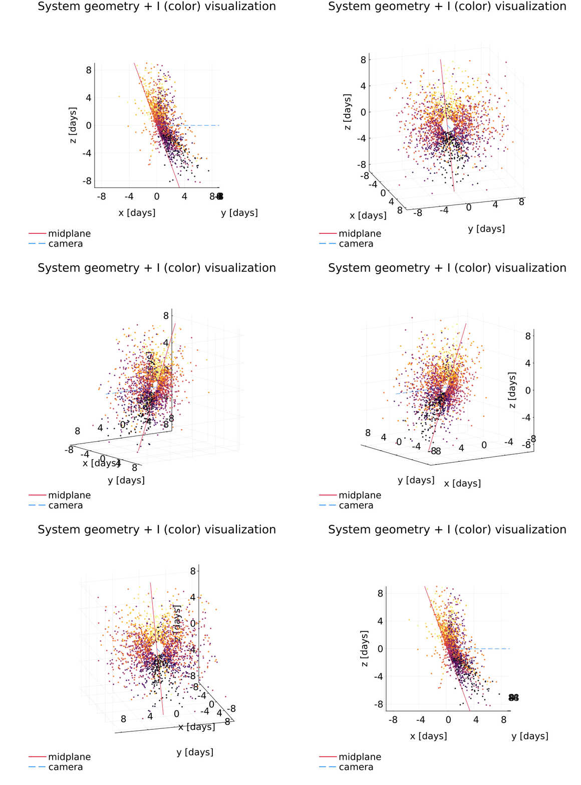 |
Comparing to the stills in Figure 4 of Pancoast+2014 again shows good agreement (note that in generating this animation the number of clouds was set to be just 2,000 to better show the structure/agreement with Pancoast+2014).
Reproducing the line and phase profiles shown in Long+2023
While reverberation mapping has historically been the primary way to constrain the properties of the BLR, advances in interferometry have recently allowed for the BLR to be directly "imaged" by GRAVITY on the VLTI, up to $z\sim 2.5$!
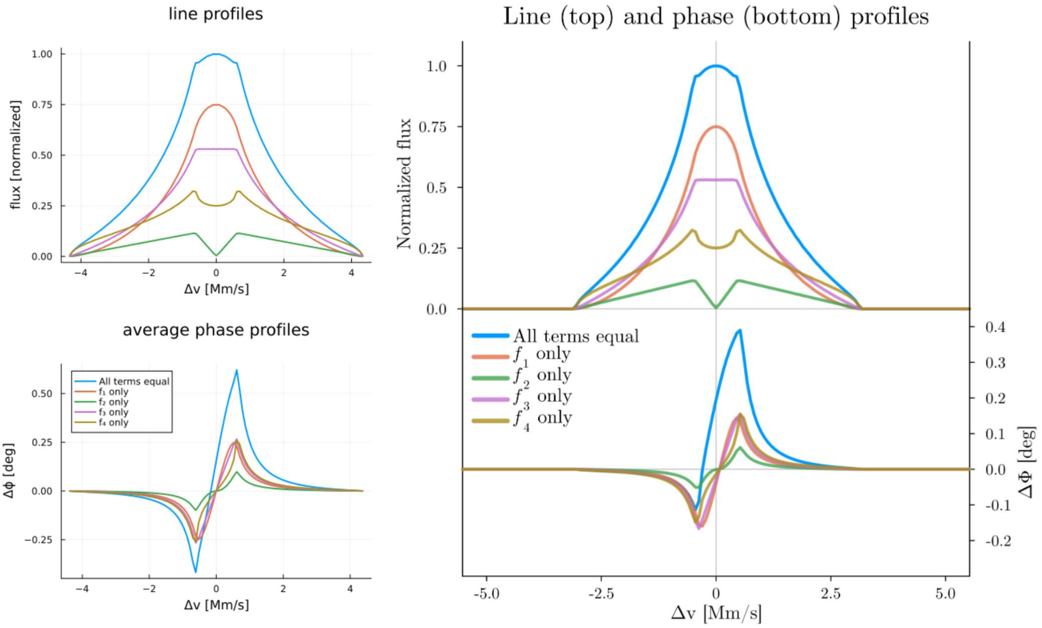
Here we will demonstrate how to generate line and phase profiles for model BLRs, reproducing the results shown in the left panel in Figure 2 of Long+2023 in the process. To start, we define disk-wind model objects for each case shown in the figure:
mLAll = BLR.DiskWindModel(8e3,45.,1.,45/180*π,nr=2048,nϕ=1024,
        I=BLR.DiskWindIntensity,v=BLR.vCircularDisk,f1=1.0,f2=1.0,
        f3=1.0,f4=1.0,τ=5.,reflect=false)
mLf1 = BLR.DiskWindModel(8e3,45.,1.,45/180*π,nr=2048,nϕ=1024,
        I=BLR.DiskWindIntensity,v=BLR.vCircularDisk,f1=1.0,f2=0.0,
        f3=0.0,f4=0.0,τ=5.,reflect=false)
mLf2 = BLR.DiskWindModel(8e3,45.,1.,45/180*π,nr=2048,nϕ=1024,
        I=BLR.DiskWindIntensity,v=BLR.vCircularDisk,f1=0.0,f2=1.0,
        f3=0.0,f4=0.0,τ=5.,reflect=false)
mLf3 = BLR.DiskWindModel(8e3,45.,1.,45/180*π,nr=2048,nϕ=1024,
        I=BLR.DiskWindIntensity,v=BLR.vCircularDisk,f1=0.0,f2=0.0,
        f3=1.0,f4=0.0,τ=5.,reflect=false)
mLf4 = BLR.DiskWindModel(8e3,45.,1.,45/180*π,nr=2048,nϕ=1024,
        I=BLR.DiskWindIntensity,v=BLR.vCircularDisk,f1=0.0,f2=0.0,
        f3=0.0,f4=1.0,τ=5.,reflect=false)
Setting the values in DiskWindModel to approximately match those in the paper.
We can then generate the line profiles for each just as we did in the CM96 example above:
LPAll = BLR.getProfile(mLAll,:line,bins=101,centered=true)
LPf1 = BLR.getProfile(mLf1,:line,bins=101,centered=true)
LPf2 = BLR.getProfile(mLf2,:line,bins=101,centered=true)
LPf3 = BLR.getProfile(mLf3,:line,bins=101,centered=true)
LPf4 = BLR.getProfile(mLf4,:line,bins=101,centered=true)
Note that this time we don't store the profiles in their respective models (although we could!) because we are going to plot all of the models on top of each other by hand.
To generate the average phase profile we need to pass a few bits of additional information to the phase function. As the documenation there shows, we must supply the U-V baseline information (in units of $\rm{M\lambda}$), the position angle, and the angular scale size of the BLR. Using the published information in the paper we can set these quantities and generate the average phase profiles like so:
#"off" axis U-V baselines as in Gravity+2019, Long+2023
U = [-14.942664391893409, -29.796334354450384, -14.76368897621181, -7.76620715016356, -11.58052554955926, -4.073062007808528, -14.957054767646966, -28.352905965208993, -13.459074151241555, -13.168981507518257, -23.464313904842403, -10.912122036718138] #Mλ
V = [-15.04195936592504, -36.26778925081391, -21.229760064196043, -14.479367253742678, -35.24862063439095, -20.773150186942956, -14.816925731069297, -35.8588243819711, -21.043799197907198, -15.401140293812933, -37.58326121804998, -21.630778375611328] #Mλ
BLRAng = 2*8e7*2e33*6.67e-8/9e20/548/3.09e24 #rₛ in radians for BLR distance of 548 Mpc
PA = 300/180*π #rad

phaseAll = BLR.getProfile(mLAll,:phase,bins=101,centered=true,U=U,V=V,PA=PA,BLRAng=BLRAng)
phasef1 = BLR.getProfile(mLf1,:phase,bins=101,centered=true,U=U,V=V,PA=PA,BLRAng=BLRAng)
phasef2 = BLR.getProfile(mLf2,:phase,bins=101,centered=true,U=U,V=V,PA=PA,BLRAng=BLRAng)
phasef3 = BLR.getProfile(mLf3,:phase,bins=101,centered=true,U=U,V=V,PA=PA,BLRAng=BLRAng)
phasef4 = BLR.getProfile(mLf4,:phase,bins=101,centered=true,U=U,V=V,PA=PA,BLRAng=BLRAng)
We can then plot the line and phase profiles for all the models and compare to Figure 2 in Long+2023:
using Plots

pLP = plot(title="line profiles",xlabel="Δv [Mm/s]",ylabel="flux [normalized]") #initialize LP plot
LPList = [LPAll,LPf1,LPf2,LPf3,LPf4]
norm = maximum(LPAll.binSums)
for p in LPList
    pLP = plot!(p.binCenters.*3e2,p.binSums./norm,label="",lw=2) #label them in the phase plot only
end

phaseList = [phaseAll,phasef1,phasef2,phasef3,phasef4]
weightedPhase = [p.binSums.*maximum(lp.binSums)./norm for (p,lp) in zip(phaseList,LPList)] #just for this figure

pPhase = plot(title="average phase profiles",xlabel="Δv [Mm/s]",ylabel="Δϕ [deg]",legend=:topleft) #initialize phase plot
labels = ["All terms equal","f₁ only","f₂ only","f₃ only","f₄ only"]
for (l,p,Δϕ) in zip(labels,phaseList,weightedPhase)
    pPhase = plot!(p.binCenters.*3e2,Δϕ.*180/π,label=l,lw=2)
end

plot(pLP,pPhase,layout=@layout([a;b]),size=(500,800),margins=5*Plots.Measures.mm)
Which should return something similar to the left panel below. Compared to the original plot (right panel) we can again see that we have well reproduced the result (although not quite exactly as seen in the height of the blue phase profile, as I no longer remember the exact set of parameters I used).
Predicting BLR sizes from differential visibility amplitudes
The differential phase profiles above encode the photocenter (first image moment) of each velocity channel, but at second order the interferometric signal also contains the size (second image moment) of the emission: in the marginally-resolved limit the line visibility amplitude dips below the continuum by $1 - |V_l| = 2\pi^2|u|^2\sigma_\theta^2$, where $\sigma_\theta$ is the rms angular extent of the channel image projected along the baseline direction. While this has not yet been measured experimentally, we include the ability to predict this quantity for various models via the secondMoment function, both per velocity channel and integrated over the entire line.
Continuing with the disk-wind model and baselines from the example above:
res = BLR.secondMoment(mLAll,bins=101,centered=true,U=U,V=V,PA=PA,BLRAng=BLRAng) #list of (edges, centers, σ², σ²tot) per baseline
edges, centers, σ², σ²tot = res[1] #σ² [rad²] per velocity channel and integrated over the line, first baseline

rad2μas = 180/π*3600*1e6
plot(centers.*3e2, sqrt.(σ²).*rad2μas, lw=2, label="",
    xlabel="Δv [Mm/s]", ylabel="rms size along baseline [μas]")
The per-channel sizes can also be generated through the usual getProfile interface with :moment2 (returning the average across baselines, like :phase does), which plugs into setProfile! and the plotting recipes:
m2All = BLR.getProfile(mLAll,:moment2,bins=101,centered=true,U=U,V=V,PA=PA,BLRAng=BLRAng)The predicted amplitude signal on a given baseline follows directly, e.g. for the first baseline:
absu = hypot(U[1],V[1])*1e6 #baseline length in units of λ
Vl = 1 .- 2π^2*absu^2 .* σ² #per-channel line visibility amplitude
Note that the line-integrated size σ²tot is not the flux-weighted average of the per-channel sizes: by the law of total variance it also contains the spread of the per-channel photocenters about the global centroid, which for a rotation-dominated BLR is comparable to the mean per-channel size. secondMoment computes it by placing the whole line in a single channel (the moment analog of averaging the complex visibilities before taking the modulus), so both terms are included automatically.
Reproducing the combined model line and delay profiles shown in Long+2025
The real utility of BroadLineRegions.jl is not in its ability to model certain prescriptions for the BLR, but instead the ability to flexibly combine them. To demonstrate this we will reproduce the hybrid disk + cloud model line and delay profiles shown in Figure 4 of Long+2025. As described in the paper, this model is a combination of a Pancoast style "cloud" model and a simple azimuthally isotropic disk model with a bit of radial inflow. We can generate both submodels and then combine them with simple syntax:
mDisk = BLR.DiskWindModel(300.,40.,1.0,30/180*π,nr=512,nϕ=1024,f1=0.0,f2=0.0,f3=0.0,f4=1.0,
        reflect=false,I=BLR.DiskWindIntensity,τ=5.,v=BLR.vCircularRadialDisk,vᵣFrac=0.33,inflow=true)
        #setting only f4 = azimuthally isotropic disk, 2/3 Keplerian 1/3 inflow velocity field
mClouds = BLR.cloudModel(1_000_000; I=BLR.cloudIntensity, v=BLR.vCloudTurbulentEllipticalFlow, i=30/180*π,
        θₒ=15/180*π, β=1.25, F=0.5, μ=300., κ=0.4, ξ=0.6, γ=0.65, fEllipse=0.8, fFlow=0.0, θₑ=35/180*π, σρᵣ=0.2,
        σρc=0.04, σΘᵣ=0.4, σΘc=0.1, σₜ=0.05,τ=0.0)
        #parameters from Long+2025

#in Long+2025 the ratio between the sum of intensity values in the cloud submodel and disk submodel is ~1:1
#so we need to rescale one of the models to ensure this is true
#note that scaling things this way is arbitrary -- a more physical way would be to specify the ratio of I*ΔA
IDisk = BLR.getVariable(mDisk,:I)
IClouds = BLR.getVariable(mClouds,:I)
ratio = sum(IDisk[.!isnan.(IDisk)])/sum(IClouds[.!isnan.(IClouds)])
for ring in mDisk.rings
    ring.I .*= 1/ratio
end
BLR.reset!(mDisk) #after mutating ring fields directly, reset! invalidates the model's cached arrays (see Performance notes in the API docs)

mCombined = mDisk+mClouds #all we have to do to combine models is "add" them!
We can again easily generate profiles for both the combined model and the submodels. This time we will generate line and delay profiles for each component and the combined model to compare to Figure 4 of Long+2025:
#get line profiles for each model
LPCombined = BLR.getProfile(mCombined,:line,minX=-1e4/3e5,maxX=1e4/3e5,bins=101)
LPDisk = BLR.getProfile(mDisk,:line,minX=-1e4/3e5,maxX=1e4/3e5,bins=101)
LPClouds = BLR.getProfile(mClouds,:line,minX=-1e4/3e5,maxX=1e4/3e5,bins=101)
#get delay profiles for each model
DPCombined = BLR.getProfile(mCombined,:delay,minX=-1e4/3e5,maxX=1e4/3e5,bins=101)
DPDisk = BLR.getProfile(mDisk,:delay,minX=-1e4/3e5,maxX=1e4/3e5,bins=101)
DPClouds = BLR.getProfile(mClouds,:delay,minX=-1e4/3e5,maxX=1e4/3e5,bins=101)

#plot the results
using Plots
pLP = plot(LPCombined.binCenters.*3e5,LPCombined.binSums./maximum(LPCombined.binSums),c=:purple,lw=2,label="")
pLP = plot!(LPDisk.binCenters.*3e5,LPDisk.binSums./maximum(LPDisk.binSums),c=:dodgerblue,lw=2,label="",ls=:dash)
pLP = plot!(LPClouds.binCenters.*3e5,LPClouds.binSums./maximum(LPClouds.binSums),c=:crimson,lw=2,label="",ls=:dash)
pLP = plot!(xlabel="v [km/s]",ylabel="flux [normalized]",title="line profiles",xticks=[0.5e4*i for i=-2:2],xlims=(-1e4,1e4))

M = 1.7e8*2e30 #kg
rs = 2*6.67e-11*M/9e16 #2GM/c^2, m
rsDay = rs/3e8/3600/24 #days
pDP = plot(DPCombined.binCenters.*3e5,DPCombined.binSums.*rsDay,c=:purple,lw=2,label="combined")
pDP = plot!(DPDisk.binCenters.*3e5,DPDisk.binSums.*rsDay,c=:dodgerblue,lw=2,label="thin-disk component",ls=:dash)
pDP = plot!(DPClouds.binCenters.*3e5,DPClouds.binSums.*rsDay,c=:crimson,lw=2,label="cloud component",ls=:dash)
pDP = plot!(xlabel="v [km/s]",ylabel="delay [days]",title="delay profiles",xticks=[0.5e4*i for i=-2:2],
    foreground_color_legend=nothing,background_color_legend=nothing,xlims=(-1e4,1e4),ylims=(0,16))

plot(pLP,pDP,layout=@layout([a;b]),size=(500,800),tickdirection=:out,minorticks=true,margins=5*Plots.Measures.mm)
Which should produce something like the left panel in the comparison below (with the right panel being the result published in Long+2025):
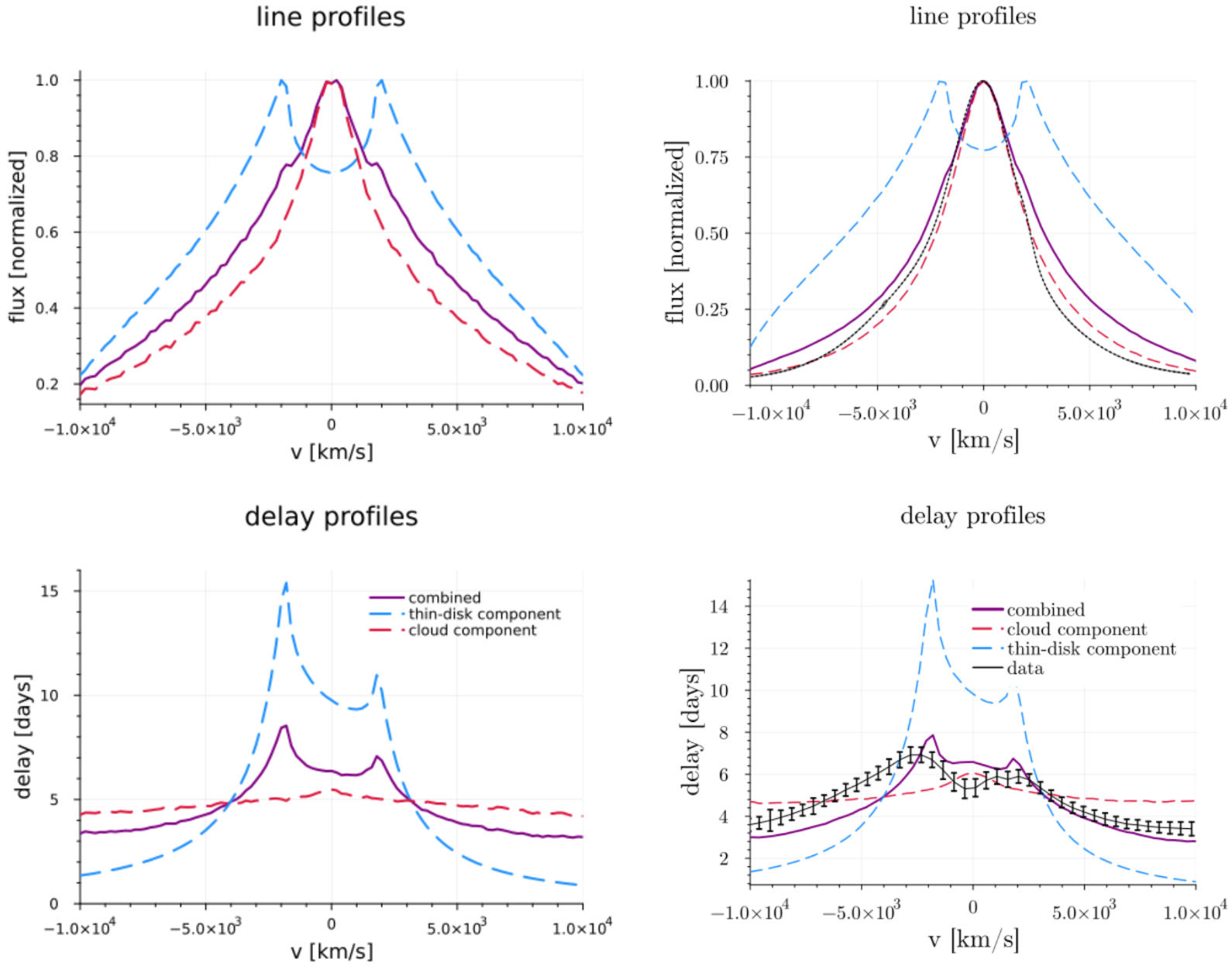
Note that there is some inherent randomness in the clouds and the width here is slightly larger than shown in the original paper to better demonstrate the two component nature, but you can improve the smoothness of the profiles by increasing the number of model points and fine tuning the width of the cloud profile if you so desire, and we've clearly reproduced the main features in the plot just fine even at this lower resolution and non fine-tuned prescription.
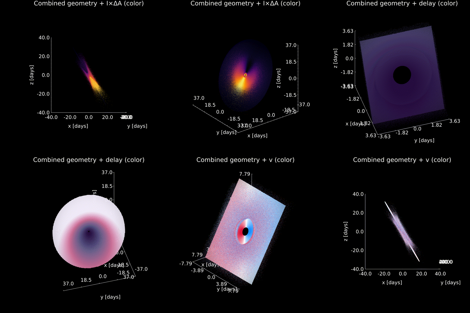
You can of course visualize your combined models with the same standard plotting recipes shown earlier to generate fun animations like the one below showcasing the intensity, delay, and velocity structure of this combined model:
Defining your own custom models
BroadLineRegions.jl makes it easy to define your own models, either by modifying one of the existing classes of models or starting entirely from scratch.
For example, say you wanted to use the cloudModel as a base but wanted the intensities to be completely randomized. You could define your own custom intensity function and pass that to the cloudModel constructor like so:
myCustomIntensityFunction(;_...) = rand() #note the _... to handle unsupported kwargs that may be passed to your intensity function
myCloudModel = BLR.cloudModel(100,I=myCustomIntensityFunction) #100 clouds with random intensities using defaults for all other parameters
It is possible to pass custom intensity, velocity, response, and optical depth functions to either cloudModel or DiskWindModel.
If you already have some precalculated result for any of the above quantities which you would like to use in your model, you can also pass that array to the model constructor so long as it matches the size requirements (i.e. if you have 100 clouds must pass an array of 100 intensities).
You can also modify models after creation, as shown in the Long+2025 example above where we rescaled the total intensity in the disk submodel.
Of course you are not limited to using BroadLineRegions.jl's predefined model constructors. The most general way to make a model is to simply pass an array of ring structs, a dictionary of profile structs, a camera struct, and an array of submodel start indices.
Each ring represents a "ring" on a "camera" observing the BLR, and this mutable structs holds all the interesting quantities about the BLR we might wish to model. The camera struct holds the $\alpha$ (x) and $\beta$ (y) camera coordinates for all points in the model, and in each corresponding ring we must supply the relevant physical information on the BLR associated with that camera pixel. See the full documentation of ring for all available options, but at a minimum in each ring we must define $\phi$, $I$, $v$, $i$ and $r$ for the BLR.
For example, say we were looking top down at an imaginary BLR whose bespoke structure happened to spell out the friendly message "don't panic" with random intensities and rotating out of the page. We could implement this custom BLR like:
# Generate a matrix with 1s for letter pixels and 0s for background
function fortytwo() #Full disclosure: Claude helped write this one...
    mat = zeros(Int, 8, 53)

    # d
    mat[1,1] = 1; mat[1,2] = 1; mat[1,3] = 1; mat[1,4] = 1
    mat[2,1] = 1;                                      mat[2,5] = 1
    mat[3,1] = 1;                                      mat[3,5] = 1
    mat[4,1] = 1;                                      mat[4,5] = 1
    mat[5,1] = 1;                                      mat[5,5] = 1
    mat[6,1] = 1;                                      mat[6,5] = 1
    mat[7,1] = 1;                                      mat[7,5] = 1
    mat[8,1] = 1; mat[8,2] = 1; mat[8,3] = 1; mat[8,4] = 1

    # o
    mat[1,7] = 1; mat[1,8] = 1; mat[1,9] = 1; mat[1,10] = 1; mat[1,11] = 1
    mat[2,7] = 1;                                            mat[2,11] = 1
    mat[3,7] = 1;                                            mat[3,11] = 1
    mat[4,7] = 1;                                            mat[4,11] = 1
    mat[5,7] = 1;                                            mat[5,11] = 1
    mat[6,7] = 1;                                            mat[6,11] = 1
    mat[7,7] = 1;                                            mat[7,11] = 1
    mat[8,7] = 1; mat[8,8] = 1; mat[8,9] = 1; mat[8,10] = 1; mat[8,11] = 1

    # n
    mat[1,13] = 1;                                           mat[1,17] = 1
    mat[2,13] = 1;                                           mat[2,17] = 1
    mat[3,13] = 1; mat[3,14] = 1; mat[3,15] = 1;             mat[3,17] = 1
    mat[4,13] = 1; mat[4,14] = 1; mat[4,15] = 1; mat[4,16] = 1; mat[4,17] = 1
    mat[5,13] = 1;                               mat[5,16] = 1; mat[5,17] = 1
    mat[6,13] = 1;                                           mat[6,17] = 1
    mat[7,13] = 1;                                           mat[7,17] = 1
    mat[8,13] = 1;                                           mat[8,17] = 1

    # ' (apostrophe)
    mat[1,19] = 1
    mat[2,19] = 1

    # t
                   mat[1,22] = 1
                   mat[2,22] = 1
    mat[3,21] = 1; mat[3,22] = 1; mat[3,23] = 1; mat[3,24] = 1; mat[3,25] = 1
    mat[4,21] = 1; mat[4,22] = 1; mat[4,23] = 1; mat[4,24] = 1; mat[4,25] = 1
                   mat[5,22] = 1
                   mat[6,22] = 1
                   mat[7,22] = 1;                                           mat[7,25] = 1
                   mat[8,22] = 1; mat[8,22] = 1; mat[8,23] = 1; mat[8,24] = 1

    # space between t and p

    # p
    mat[1,29] = 1; mat[1,30] = 1; mat[1,31] = 1; mat[1,32] = 1; mat[1,33] = 1
    mat[2,29] = 1;                                           mat[2,33] = 1
    mat[3,29] = 1;                                           mat[3,33] = 1
    mat[4,29] = 1; mat[4,30] = 1; mat[4,31] = 1; mat[4,32] = 1; mat[4,33] = 1
    mat[5,29] = 1
    mat[6,29] = 1
    mat[7,29] = 1
    mat[8,29] = 1

    # a
    mat[1,35] = 1; mat[1,36] = 1; mat[1,37] = 1; mat[1,38] = 1; mat[1,39] = 1
    mat[2,35] = 1;                                           mat[2,39] = 1
    mat[3,35] = 1;                                           mat[3,39] = 1
    mat[4,35] = 1; mat[4,36] = 1; mat[4,37] = 1; mat[4,38] = 1; mat[4,39] = 1
    mat[5,35] = 1; mat[5,36] = 1; mat[5,37] = 1; mat[5,38] = 1; mat[5,39] = 1
    mat[6,35] = 1;                                           mat[6,39] = 1
    mat[7,35] = 1;                                           mat[7,39] = 1
    mat[8,35] = 1;                                           mat[8,39] = 1

    # n
    mat[1,41] = 1;                                           mat[1,45] = 1
    mat[2,41] = 1;                                           mat[2,45] = 1
    mat[3,41] = 1; mat[3,42] = 1; mat[3,43] = 1;             mat[3,45] = 1
    mat[4,41] = 1; mat[4,42] = 1; mat[4,43] = 1; mat[4,44] = 1; mat[4,45] = 1
    mat[5,41] = 1;                               mat[5,44] = 1; mat[5,45] = 1
    mat[6,41] = 1;                                           mat[6,45] = 1
    mat[7,41] = 1;                                           mat[7,45] = 1
    mat[8,41] = 1;                                           mat[8,45] = 1

    # i
    mat[1,47] = 1
    mat[3,47] = 1
    mat[4,47] = 1
    mat[5,47] = 1
    mat[6,47] = 1
    mat[7,47] = 1
    mat[8,47] = 1

    # c
    mat[1,49] = 1; mat[1,50] = 1; mat[1,51] = 1; mat[1,52] = 1; mat[1,53] = 1
    mat[2,49] = 1
    mat[3,49] = 1
    mat[4,49] = 1
    mat[5,49] = 1
    mat[6,49] = 1
    mat[7,49] = 1
    mat[8,49] = 1; mat[8,50] = 1; mat[8,51] = 1; mat[8,52] = 1; mat[8,53] = 1

    return mat
end

mat = reverse(fortytwo(),dims=1) #reverse top/bottom
α = zeros(sum(mat)) #camera x coordinates in units of rs
β = zeros(sum(mat)) #camera y coordinates in units of rs
αj = range(-size(mat)[2]/2,stop=size(mat)[2]/2,length=size(mat)[2])
βi = range(-size(mat)[1]/2,stop=size(mat)[1]/2,length=size(mat)[1])
counter = 0
for i=1:size(mat)[1]
    for j=1:size(mat)[2]
        if mat[i,j] != 0 #fill in camera coordinates where matrix non-empty
            counter += 1 #which point are we on?
            α[counter] = αj[j]
            β[counter] = βi[i]
        end
    end
end

cam = BLR.camera(α,β,false) #initialize the camera for the model, set raytraced flag to false

rings = Array{BLR.ring}(undef,sum(mat)) #initialize array of rings

for j=1:length(rings) #define the rings with minimum physical quantities of our model BLR
    r = √(α[j]^2+β[j]^2) #radius in physical space = camera radius for i = 0.0
    ϕ = atan(β[j],α[j]) #angle in physical space = camera ngle for i = 0.0
    i = 0.0 #inclination
    I = rand()
    v = sqrt(1/r)*sign(α[j]) #rotating in/out of the page and proportional to √1/r
    ΔA = 1.0 #rₛ²
    rings[j] = BLR.ring(r=r,ϕ=ϕ,i=i,I=I,v=v,ΔA=ΔA) #define ring with minimum physical quantities using defaults for everything else
    #note that 3d plotting will be wrong for this, as the 3D plotting routine assumes you start with point in x-y plane and then rotate into z direction
    #do things in this order if you care about 3d visualizations of your custom models (but otherwise it does not matter)
end

# Create the custom BLR model
myCustomModel = BLR.model(rings,Dict{Symbol,BLR.profile}(),cam,[1]) #no profiles (yet), only one submodel so subModelStartInds = [1]

#visualize it
using Plots
imgI = BLR.image(myCustomModel,:I,markersize=2.,background_color=:black,cmap=cgrad([:red,:lime],[0.0,0.3,1.0]))
imgv = BLR.image(myCustomModel,:v,markersize=2.,background_color=:black,cmap=cgrad([:blue,:red],[-1.,0.,1.]))
p = BLR.getProfile(myCustomModel,:line,bins=10)
BLR.setProfile!(myCustomModel,p)
p = BLR.getProfile(myCustomModel,:r,bins=10)
BLR.setProfile!(myCustomModel,p)
p = BLR.getProfile(myCustomModel,:ϕ,bins=10)
BLR.setProfile!(myCustomModel,p)
P = BLR.profile(myCustomModel)
plot(imgI,imgv,P,layout=@layout([grid(2,1) P{0.4w}]),size=(800,400),margins=5*Plots.Measures.mm)
Which produces the following plot: 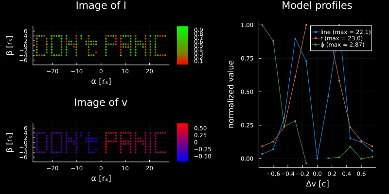
If you want the default 3D visualizations to work correctly, define your points in the x-y plane and then rotate them into 3D space using rotate3D as this is what plot3d calls on points to make the 3D visualizations. This should not affect any science use case if you opt to initialize the points some other way (like in the quick example above).
Multi-line models
Everything above models the BLR for a single broad emission line, but of course the BLR often has multiple broad emission lines we might want to model concurrently. This is easily accomplished in BroadLineRegions.jl given its flexibility, and we provide a nice wrapper to support this process with the CompositeModel type. This is simply a custom type that holds several models at once, with each BLR model given a unique name, central wavelength, and relative flux normalization to signify it represents a distinct emission line. The per-line models stay completely independent — combining lines this way changes nothing about how each individual model behaves, and importantly each line model can itself be a multi-component BLR model as described above, so as much complexity as you want is possible in this way.
To create a multi-line BLR model, simply start with an existing single line BLR model and add it to a CompositeModel:
mHα = BLR.DiskWindModel(3000.,100.,1.,75/180*π,
        nr=2048,nϕ=1024,scale=:log,f1=1.0,f2=1.0,f3=0.0,f4=0.0,
        I=BLR.DiskWindIntensity,v=BLR.vCircularDisk,τ=5.0,reflect=false) #say the Hα line is modeled by a simple DiskWind model with this parameterization
cm = BLR.CompositeModel(mHα; line="Hα", lineCenter=6563.) #initialize the composite model, labeling the Hα line and denoting its line center in whatever units you prefer -- but note BroadLineRegions.jl is not aware of these units, so each subsequent line added must use the same units.
lineCenter units are arbitrary (Å above, but nm/μm/anything works) — the only requirement is that they are mutually consistent across all lines in one CompositeModel, since only the ratio of Δλ/λ matters. This is your responsibility to manage and is not checked by the code.
Once you have initialized your CompositeModel, there are two ways to add more lines with addLine!. You can pass an explicitly constructed separate model like:
mCIV = BLR.cloudModel(1_000_000; μ=1000.0, β=1.0, F=0.5, θₒ=30/180*π, i=30/180*π, γ=1.0, ξ=1.0,
        I=BLR.cloudIntensity, v=BLR.vCircularCloud, τ=5.0, rng=:philox, seed=42) #completely independently constructed BLR model with its own distinct parameters
BLR.addLine!(cm, mCIV; line="CIV", lineCenter=1549., fluxRatio=0.8) #now the CompositeModel cm holds both the DiskWindModel from before for Hα and this new CIV cloud model
Alternatively, you can also reuse the recorded construction parameters of any existing BLR model that has already been added to the CompositeModel (via rebuild on model.params), overriding only what should differ:
BLR.addLine!(cm; line="Hβ", lineCenter=4861., fluxRatio=0.35, from="Hα", r̄=2000.) #all parameters the same as the Hα line model, except move r̄ in from 3000 -> 2000 rₛHere fluxRatio is the line's velocity-integrated flux relative to the first line in the CompositeModel (in this example "Hα" ≡ 1.0), so the semantics are independent of each intensity function's arbitrary units. Line models are identical except for the central wavelength and flux normalization in this way unless an override parameter is specified (like we did in this example for r̄), and if one is specified the new model is built internally the same way you would build it yourself on the outside — this wrapper just provides more convenient syntax/saves a bit of typing.
A note on seeds: cloud models built with rng=:philox, seed=... (like mCIV above) rebuild bit-identically under parameter reuse — the stored seed is reused unless you override it, so an addLine!(cm; from="CIV", ...) line samples "clouds" identically as the first line. Pass a new seed to draw fresh (statistically equivalent but different) cloud points. Models built with the legacy AbstractRNG path cannot be reproduced exactly (the RNG state was consumed) and warn accordingly.
We can obtain the combined wavelength-space spectrum for our new multi-line BLR CompositeModel using getSpectrum, which can be visualized directly with the spectrum plotting recipe (one series per line plus the total, with any overlapping line regions shaded):
edges, centers, flux, total = BLR.getSpectrum(cm; bins=200) #the underlying data; sum(flux[line]) == fluxRatio
BLR.spectrum(cm; bins=200) #plot it (pass z=... to shift to the observed frame, but note here we already used the line central wavelengths at z=0)
Whether lines overlap in wavelength space can be checked with lineOverlap, which returns one (lineA, lineB, λlo, λhi) entry per overlapping pair (an empty vector means no overlaps):
BLR.lineOverlap(cm) #NamedTuple[] here -- Hα/Hβ/CIV are far apart compared to their velocity widthsOf course all the usual single-model entry points work per line on this new CompositeType as you would expect, i.e. BLR.getProfile(cm, :line; line="Hβ"), BLR.getVariable(cm, :r; line="CIV"), BLR.raytrace!(cm), BLR.image(cm, :I; line="Hα"), BLR.plot3d(cm), and BLR.profile(cm) (which overlays every line's profile).
Velocities map to wavelengths at first order, λ = lineCenter*(1+v) (see wavelength), with the stored line-of-sight velocity v in units of c.
Velocity-resolved line ratios
With several lines in one CompositeModel we can also model the velocity-resolved ratio of any two of them, i.e. the Balmer decrement BD(v) = FHα(v)/FHβ(v), for example recently measured for a sample of "Little Red Dots" in Chen et al. 2026 (§5.3). This quantity is simply the ratio of the two continuum-subtracted broad-line profiles interpolated onto a common velocity grid, which we can calculate from our CompositeModel with the getProfile(cm, :ratio; lines=(a, b)) method. This bins the fluxes from both lines onto shared velocity bins and divides, returning a profile struct named Symbol("a/b").
As a simple example, consider two Balmer series lines modeled as DiskWindModels in BroadLineRegions.jl with different radial emissivity profiles:
mHα = BLR.DiskWindModel(7500., 100., 1., 75/180*π; nr=2048, nϕ=4096, scale=:log,
        I=BLR.DiskWindIntensity, v=BLR.vCircularDisk, f1=1.0, f2=1.0, f3=0.0, f4=0.0,
        τ=5.0, reflect=false) # a simple disk-wind model that will have a singly peaked line profile, power-law source function α = 1
cm = BLR.CompositeModel(mHα; line="Hα", lineCenter=6563.) #initialize the CompositeModel

BLR.addLine!(cm; line="Hβ", lineCenter=4861., fluxRatio=1/2.86, from="Hα", α=1.25, r̄=5000.) #Case B integrated decrement
# Hβ reuses all the parameters from Hα but with a steeper power-law and different intensity-weighted mean radius to compensate for this
# steeper power-law such that the radial grids are roughly the same size in both Hα and Hβ
c_kms = 2.99792458e5
vEdges = collect(-2500.:100.:2500.) ./ c_kms #use 100 km/s bins between -2500 and 2500 km/s, converted to units of c
bd = BLR.getProfile(cm, :ratio; lines=("Hα", "Hβ"), bins=vEdges) #the velocity-resolved Balmer decrement BD(v)
BLR.profile(cm)   #both line profiles, overlaid
BLR.profile(bd)   #BD(v) itself -- centrally peaked, declining toward the wings
# equivalently, plot straight from the composite without computing `bd` first (the lines pair is
# positional here because Plots reserves `lines` as a keyword): BLR.profile(cm, :ratio, ("Hα", "Hβ"))
This example was chosen to get the shape of the BD(v) profile to roughly match what was observed and described in Chen+ 2026, where they observed Balmer decrements with ~single peaks and decreasing roughly by a factor of two between the center and the wings. Of course this is a very simple example, and many further complications are possible, including passing your own custom intensity functions as described in earlier sections of the documentation.
An important subtlety of the integrated-flux semantics: each line's profile is normalized to unit integral before being scaled by its fluxRatio, so any constant prefactor on a line's intensity divides out — the per-line model sets only the velocity shape of BD(v), while the integrated decrement is pinned by fluxRatio alone (so you can scale it any way you like after generation). This means that there could be a discrepancy between the "real" ratio in between the two models and the ratio shown in the plot, but of course if you would rather let the per-line models themselves set the integrated decrement without pinning it by hand, you can compute the fluxRatio from them directly:
IΔA(m) = sum(x for x in BLR.getVariable(m, :I, flatten=true) .* BLR.getVariable(m, :ΔA, flatten=true) if isfinite(x))
mHβ = BLR.rebuild(mHα.params; α=1.25, r̄=5000.) #the same model addLine! builds internally
cm2 = BLR.CompositeModel(mHα; line="Hα", lineCenter=6563.)
BLR.addLine!(cm2, mHβ; line="Hβ", lineCenter=4861., fluxRatio=IΔA(mHβ)/IΔA(mHα)) #model-implied integrated decrement
The integrated ratio of any two registered lines is always available as lineRatio(cm, "Hα", "Hβ") (== fluxRatios["Hα"]/fluxRatios["Hβ"] by the semantics above).
Running on the GPU
As of version 0.3.0, BroadLineRegions.jl can now generate/port models to a GPU for significant performance gains on some workflows. NVIDIA GPUs are supported through CUDA.jl, and as of version 0.4.1 Apple-silicon Macs are supported through Metal.jl. The GPU kernels are shared, so everything on this page works with both. Below we repeat the CM96 example from above showcasing how to access these capabilities and the kind of performance gains one might expect from using BroadLineRegions.jl on your GPU. First, we must load a GPU backend (CUDA.jl for NVIDIA devices and Metal.jl for Apple Silicon) alongside BroadLineRegions to enable these features:
using BroadLineRegions
using CUDA #or using Metal, if you are on a Mac and want to use Apple Silicon GPUThe GPU entry points default to Float32 (T=Float32) because consumer (GeForce) cards run Float64 at roughly 1/64 the Float32 rate. Float32 is plenty for most line-profile and transfer-function work; pass T=Float64 if you are on a data-center card or need the extra precision. Apple Silicon can only support Float32 so passing Float64 will error on a Mac if trying to use the GPU.
After loading whatever package (CUDA/Metal) is relevant for your hardware, with simple syntax (that is agnostic to GPU backend) we can now port our models and many of our calculations to the GPU. To replicate the CM96 disk model example from the beginning of these docs with calculations now done on the GPU we just need a tiny bit of extra new syntax. Shown below are two ways to get this CM96 model onto the GPU instead of the CPU:
(1) Build on the CPU, then transfer. Construct the model exactly as before and hand it to gpu, which returns a device-resident handle you can call the observable functions on directly:
mCM96 = BLR.DiskWindModel(3000.,100.,1.,75/180*π,
        nr=2048,nϕ=1024,scale=:log,f1=1.0,f2=1.0,f3=0.0,f4=0.0,
        I=BLR.DiskWindIntensity,v=BLR.vCircularDisk,τ=5.0,reflect=false) #same as before

mGPU = BLR.gpu(mCM96)                 #device-resident handle (ModelArrays on the GPU)
p = BLR.getProfile(mGPU, :line, bins=101)
tEdges = collect(range(0.0,stop=20.0/rsDay,length=101)) #will generate 100 bins, convert 20 days upper limit to units of rs
vEdges = collect(range(-0.04,stop=0.04,length=101)) #0.04c ~12*1e8 cm/s
Ψ = BLR.getΨ(mGPU, vEdges, tEdges) #same vEdges/tEdges as the CM96 exampleWith no backend keyword the GPU functions use defaultGPUBackend(): CUDA if CUDA.jl is loaded and functional, otherwise Metal. To force one, pass it explicitly, e.g. BLR.gpu(m; backend=Metal.MetalBackend()). Time GPU work with Metal.@sync (instead of CUDA.@sync). Random cloud draws (gpuCloudModel) come from counter-based Philox substreams whose integer output is bit-identical on the CPU, CUDA, and Metal backends, so the same seed gives the same clouds on every device to Float32 rounding (a few per 10⁴ can differ where device math rounding flips a rejection-sampling decision).
The handle is built once and reused across as many observable calls as you like — nothing is re-flattened or re-copied per call. Results come back as ordinary host arrays/profiles, identical in shape to the CPU versions. You can call any observable/raytrace! on the model and will see a performance gain for each of these common function calls that can exploit the GPU. But note that you do pay a penalty to transfer the model from the CPU to the GPU, thus to see performance gains in this kind of scenario requires that the models be large (such that calculating observables/raytracing takes a long time on the CPU) or that you calculate many quantities after model creation (i.e. calling getProfile many times).
(2) Build directly on the device. For the built-in DiskWind/cloud model physics you can skip the host model entirely and construct everything instead directly on the GPU with gpuDiskWindModel (note there similarly exists a gpuCloudModel function as well). This is the fastest path for fitting where models are constantly reconstructed from new parameters, since it never allocates host rings, flattens, or transfers. To generate the same example as before but on GPU directly we thus can write:
mGPU = BLR.gpuDiskWindModel(3000.,100.,1.0,75/180*π;          #(r̄, rFac, α, i) as in CM96
        nr=2048,nϕ=1024,scale=:log,f1=1.0,f2=1.0,f3=0.0,f4=0.0,τ=5.0)
p = BLR.getProfile(mGPU, :line, bins=101)
tEdges = collect(range(0.0,stop=20.0/rsDay,length=101)) #will generate 100 bins, convert 20 days upper limit to units of rs
vEdges = collect(range(-0.04,stop=0.04,length=101)) #0.04c ~12*1e8 cm/s
Ψ = BLR.getΨ(mGPU, vEdges, tEdges) #same vEdges/tEdges as in the CM96 example
If for some reason you want the model back on the CPU, this can easily be accomplished with:
mCPU = BLR.cpu(mGPU)But note that in doing so this model object will hold the flattened array shape required to build it on the GPU and not the standard ring structs used on models created on the CPU.
How much of a performance gain does this get us? We can time the end-to-end "build a model and get its line profile" for each approach (use CUDA.@sync so the GPU work actually completes before the timer stops):
#CPU only: build host model + profile
@time begin
    m = BLR.DiskWindModel(3000.,100.,1.,75/180*π,nr=2048,nϕ=1024,scale=:log,
            f1=1.0,f2=1.0,f3=0.0,f4=0.0,τ=5.0)
    BLR.getProfile(m, :line, bins=101)
end

#GPU, build-on-device: build resident model + profile
@time CUDA.@sync begin
    mGPU = BLR.gpuDiskWindModel(3000.,100.,1.0,75/180*π;nr=2048,nϕ=1024,scale=:log,
            f1=1.0,f2=1.0,f3=0.0,f4=0.0,τ=5.0)
    BLR.getProfile(mGPU, :line, bins=101)
end
On a laptop with an AMD Ryzen 9 HX 370 CPU and RTX 5070 Ti GPU for this scenario (nr=2048, nϕ=1024, total grid size ≈ 2.1M points, 101-bin :line profile, Julia 1.12), the measured wall-clock times are:
| approach | time | vs. CPU-only |
|---|---|---|
CPU only — build + getProfile(:line) | ~360–720 ms | 1× |
GPU, build-on-device (gpuDiskWindModel) + profile, Float32 | ~2.2 ms | ~160–330× |
GPU, build-on-device + profile, Float64 | ~7.5 ms | ~50–95× |
So building directly on the device is well over two orders of magnitude faster for this build-dominated work (Float32), and the gap grows with nr/nϕ and with the number of clouds — most of the win is eliminating the host build + flatten + transfer, not just the kernel compute. (The CPU time varies run-to-run by roughly 2× here, which is where the spread in the speedup column comes from; regenerate on your own hardware. All times are warm/steady-state — the first call in a fresh session additionally pays one-time kernel compilation.)
gpu(m) (approach 1) is not a shortcut if you are only going to take a single profile of a newly built model — building the host model, flattening it, and copying it to the device costs more than just evaluating the profile on the CPU (≈ 4 s here, slower than CPU-only). Its value is reuse: once a model is resident on the GPU, each additional observable call is at least ~15× faster than the equivalent CPU implementation. Thus use gpu(m) when you will make many observable calls on one model, or when trying to implement custom physics that are not easily ported to the GPU; otherwise just use gpuDiskWindModel/gpuCloudModel when you rebuild "standard" geometries every iteration.
Custom intensity / velocity on the GPU
gpuDiskWindModel accepts custom physics, as long as it can run inside a kernel — pass intensity (or velocity) as a GPU-safe scalar callable (r, ϕ, inc) -> value that closes only over isbits values. For example, for a disk with uniform emissivity (every point set to 1):
mGPU = BLR.gpuDiskWindModel(3000.,100.,1.0,75/180*π;nr=2048,nϕ=1024,scale=:log,
        intensity = (r,ϕ,inc) -> 1.0f0,    # GPU-safe scalar I(r,ϕ,inc); use 1.0f0 for Float32
        τ=5.0)
p = BLR.getProfile(mGPU, :line, bins=101)
A general Function that cannot run in a kernel (closures over arrays, calls into non-GPU libraries, etc.) should instead be used to build the model on the CPU and then moved over with BLR.gpu(m). For a more detailed worked example of the (r, ϕ, inc) -> value form to model your own physics on, see the built-in GPU-safe closures: _rt_disk_intensity_fn (the device intensity, a direct port of the CPU DiskWind_I_) and _rt_disk_velocity_fn / _rt_disk_radial_velocity_fn for an example velocity calculation.
Summary of everything else that works on the GPU
The device-resident handle is a drop-in for the observables described above: getProfile (:line, :delay, :r, :ϕ, :phase, :moment2), getΨ, getΨt, phase, and secondMoment all have methods on it, which work automatically just as they would on a CPU hosted model and with the same syntax. Combined models work too: build each submodel on the device (or copy them there) and add them with + (e.g. BLR.gpuDiskWindModel(...) + BLR.gpuCloudModel(...)) just as before, then raytrace! the combined model if desired — all without leaving the GPU. Bring any handle back to the host with BLR.cpu(mGPU). Two caveats on the resident GPU paths: they require uniform bin edges (pass an Int bin count or uniformly spaced edges), and do not accept a custom dx integration element — use the host model for those. See gpu, gpuDiskWindModel, gpuCloudModel, and residentDiskWindModel/residentCloudModel (CPU-backend builds, handy for testing the pipeline without a GPU) in the API for the full set of options.
Additional (selected) helpful tools from the API not described above
After combining submodels, access their constituent parts by simply writing:
mCombined = m1+m2 #combine two models
m1 = mCombined[1]; m2 = mCombined[2] #get access to the submodels with indexing
If you are annoyed with the output statements after things, suppress them by placing a semicolon after:
mCombined; #suppresses outputOther functions:
BroadLineRegions.getVariable — Function
getVariable(m::model, variable::Union{String,Symbol,Function}; flatten=false)Retrieve elements from model object and stack them into matrices for easy manipulation.
Arguments
m::model: Model object to extract variables fromvariable::Union{String,Symbol,Function}: Variable to extract from model- If
String, will be converted toSymbol - Must be a valid attribute of
model.rings(e.g.:I,:v,:r,:i,:ϕ) or a function that can be applied tomodel.rings - Example: Keplerian disk time delays could be calculated like
t(ring) = ring.r .* (1 .+ sin.(ring.ϕ) .* ring.i)
- If
flatten::Bool=false: If true, flatten the result to a vector
Returns
Array{Float64,}: Matrix or vector of extracted variable frommodel.rings, created by stacking the output variable for each ring- For example, if variable given is
:I, result will have shape(length(r), length(ϕ))as at eachrandϕthere is a value ofI - If
flatten=true, result will be a flattened vector
- For example, if variable given is
getVariable(m::model, variable::Symbol; flatten=false)Retrieve model variable when specified as a Symbol. See main docstring for details.
getVariable(m::model, variable::Function; flatten=false)Retrieve model variable when specified as a Function. See main docstring for details.
Note
Results are memoized in m.cache only for the package's own pure delay functions (t, tDisk, tCloud) — user-supplied functions are always re-evaluated, since they may capture state the cache cannot see.
getVariable(rm::ResidentModel, variable::Union{String,Symbol}) -> VectorHost copy of a single flat ModelArrays column by name (e.g. :I, :v, :α). This is the recipe-facing counterpart of getVariable(::model, …); the columns are already flat so it takes no flatten keyword, and it does not accept a Function (compute custom quantities on the host model). When the columns live on the GPU the result is copied back to the host.
getVariable(cm::CompositeModel, variable; line::String, flatten=false)Per-line forwarding of getVariable: gather variable from the model registered under line.
BroadLineRegions.raytrace! — Function
raytrace!(cm::CompositeModel; line=nothing, kwargs...) -> cmPer-line forwarding of raytrace!. line=nothing (the default) raytraces every line; otherwise only the named line.
raytrace! returns a new model (it does not mutate its argument), so this reassigns cm.models[line] = raytrace!(cm.models[line]; kwargs...). Lines that raytrace! would warn about and hand back unaltered – a single-submodel model (subModelStartInds == [1]) or an already-raytraced one (camera.raytraced) – are skipped silently so a multi-line loop does not warn-spam.
Raytracing happens within each line's own submodels only. Cross-line occlusion is deliberately not modeled: different lines are at different wavelengths and each line's τ is that line's own optical depth (see the Workstream-4 plan, "Out of scope").
raytrace!(m::model; IRatios::Union{Float64,Array{Float64,}}=1.0,
        τCutOff::Float64=1.0, raytraceFreeClouds::Bool=false,
        backend=nothing, T=Float64)
Perform raytracing for a model, combining overlapping components along line of sight.
This function should be called after combining all relevant models (i.e. mCombined = m1 + m2 + m3...). Points are binned by pixel, sorted front-to-back along the line of sight, and combined with a segmented exp(-τ) scan: each point attenuates those behind it, points past τCutOff are dropped, and IRatios is applied as a global per-submodel weight. A new model object is returned with the extraneous points removed. Note that this function will mutate the input model objects.
The bin→sort→segmented-scan implementation is far faster than the original brute-force raytracer (and can also run on a device via backend). If you only need simple disk obscuration removal rather than full attenuation, removeDiskObscuredClouds! is a lighter alternative.
Arguments
m::model: Model to raytraceIRatios::Union{Float64,Array{Float64,}}=1.0: Global emissivity weights for each submodel- If
Float64, applies to all submodels equally - If array, applies to each submodel individually (must match number of submodels)
- Used when combining models with different intensity functions if they aren't properly normalized
- If
τCutOff::Float64=1.0: Maximum optical depth to raytrace to (stops whenτ > τCutOff)raytraceFreeClouds::Bool=false: Whether to raytrace free clouds (cloud-cloud raytracing)- If
false, clouds are only raytraced if they overlap with a continuous model - If
true, clouds will be checked for overlap with other clouds and raytraced accordingly
- If
backend=nothing: OptionalKernelAbstractionsbackend to run the bin→sort→scan on a device.- If
nothing, uses the CPU implementation. - Pass
CUDABackend()(with CUDA.jl loaded) orMetalBackend()(with Metal.jl loaded; requiresT=Float32) to run on the GPU; see alsogpu. - Apple Silicon (Metal) GPUs have no
Float64, andTdefaults toFloat64, so passT=Float32withMetalBackend()or it errors. - On Metal the (pixel, depth) sort runs on the host (Metal.jl cannot
sortpermtuples on the device); the order is identical to the CPU/CUDA paths and the copy is cheap on unified memory.
- If
T=Float64: Element type for the device arrays whenbackendis set (useFloat32on GeForce GPUs for speed).
Returns
m::model: Model with raytraced points
raytrace!(rm::ResidentModel; IRatios=1.0, τCutOff=1.0, raytraceFreeClouds=false) -> ResidentModelDevice-resident dispatch of raytrace!: run the full bin→sort→segmented-scan→ compact combine on rm's backend with no host round-trips, returning a freshly raytraced ResidentModel (drop-in for the observable methods). rm must carry raytrace metadata — build it with gpu(m) (CUDA or Metal loaded) or resident(m; raytrace=true).
Like raytrace!(::model) this returns a new combined handle rather than mutating in place (the point count changes: one combined point per active output pixel + surviving free clouds), so write rm = raytrace!(rm). Semantics match the host raytrace!: IRatios is a global per-submodel weight, τCutOff the optical-depth cutoff, raytraceFreeClouds enables cloud–cloud attenuation.
BroadLineRegions.reset! — Function
reset!(m::model; profiles=true, img=false)Erase existing profiles/raytrace status and invalidate the model's getVariable cache.
Call this after mutating ring fields directly (e.g. m.rings[1].I .= ...) so that subsequent getVariable/getProfile calls see the new values instead of memoized ones.
Parameters
m::model: Model object to resetprofiles::Bool=true: If true, reset profilesimg::Bool=false: If true, reset raytracing boolean (does not change existing model but allows model to be raytraced again after combining other new models)
reset!(cm::CompositeModel; line=nothing, profiles=true, img=false) -> cmPer-line forwarding of reset!. line=nothing (the default) resets every line; otherwise only the named line. Extra keywords (profiles, img) forward to the per-line model method.
BroadLineRegions.phase — Function
phase(m::model; U, V, PA, BLRAng, returnAvg=false, offAxisInds=nothing, kwargs...)Calculate differential phase signal for a model based on specified baselines, model orientation, and BLR angular size.
Arguments
m::model: Model object to calculate phase forU::Vector{Float64}: U component of complex visibility in [Mλ]V::Vector{Float64}: V component of complex visibility in [Mλ]PA::Float64: On-sky position angle of the model in radiansBLRAng::Float64: Characteristic size of the BLR model in radians (conversion from $r_s$ to radians)returnAvg::Bool=false: Iftrue, returns the average phase across all baselinesoffAxisInds::Union{Nothing,Vector{Int}}=nothing: If provided, only calculates phase for baselines at specified indices
Returns
- If
returnAvg=true:Tuple{Vector{Float64},Vector{Float64},Vector{Float64}}containing:- Bin edges for velocity
- Bin centers for velocity
- Average differential phase (in radians)
- If
returnAvg=false:Vector{Tuple{Vector{Float64},Vector{Float64},Vector{Float64}}}containing:- For each baseline, a tuple of bin edges, bin centers, and differential phase
The differential phase is calculated by integrating the phase over the model at each velocity bin, weighted by the intensity and area of each ring element.
A device-resident method (phase(::ResidentModel, …)) runs this on the GPU without re-flattening the model each call; see gpu and ResidentModel.
phase(rm::ResidentModel; U, V, PA, BLRAng, returnAvg=false, offAxisInds=nothing, bins=100, kwargs...)GPU-resident differential phase, matching phase(::model, …).
BroadLineRegions.DRW — Function
function DRW(;t::Array{Float64}=collect(range(0,stop=100,length=1001)), μ::Float64=0.0, τ::Float64=1.0, σ::Float64=0.1)Generate a damped random walk continuum lightcurve following MacLeod+2010
Arguments:
t::Vector{Float64}`: time array that returned lightcurve will be sampled atμ::Float64: mean value of random walkτ::Float64: characteristic time scale of random walkσ::Float64: standard deviation of random walk
Returns:
C::Vector{Float64}: damped random walk array corresponding to times t
BroadLineRegions.syntheticLC — Function
function syntheticLC(Ct,CLC,Ψτ;tStart=0.0,normalize=false)Generate a synthetic lightcurve from a continuum lightcurve and a 1D transfer function.
Arguments:
Ct::Vector{Float64}: time array for the continuum lightcurveCLC::Vector{Float64}: continuum lightcurve values at timesCtΨτ::Vector{Float64}: transfer function values at timesCttStart::Float64: time after which the lightcurve should be normalized to zeronormalize::Bool: whether to normalize the lightcurve to the extent of variations in the continuum
Returns:
Δlc::Vector{Float64}: synthetic lightcurve sampled at timesCtwith zero point ~attStartand optionally normalized